library(tidyverse)
library(janitor)Basic data analyses
In this tutorial, we will show you how to sort and filter the data. We will also train how to append traits, indicator values or information about the status of species and calculate proportions of selected plant groups, community weighted and unweighted means or other summary statistics. If you are interested in a more general overview of the functions, you are encouraged to check also our study materials here.
2.1 Data import
We will play a bit with measured variables from our plots and try few useful functions. For more see study materials and links there. We will first read the data newly, to be sure we know what we are working with. At this point we can actually clean the environment, remove everything.
2.1.1 env dataset
First I want to add some more variables that were measured separately.
env_extra<- read_csv("data/env_measured.csv")Rows: 65 Columns: 22
── Column specification ────────────────────────────────────────────────────────
Delimiter: ","
chr (1): forest_type_name
dbl (21): releve_nr, forest_type, herbs, juveniles, coverE1, biomass, soil_d...
ℹ Use `spec()` to retrieve the full column specification for this data.
ℹ Specify the column types or set `show_col_types = FALSE` to quiet this message.For the env dataset, I want to import the clean version saved in the previous script. I will directly add selected information from the other file. For more on joins, see the study materials.
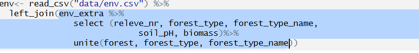
env<- read_csv("data/env.csv") %>%
  left_join(env_extra %>%
               select (releve_nr, forest_type, forest_type_name,                                                soil_pH, biomass)%>%
               unite(forest, forest_type, forest_type_name))
Rows: 65 Columns: 18
── Column specification ────────────────────────────────────────────────────────
Delimiter: ","
chr (5): coverscale, field_nr, country, author, locality
dbl (12): releve_nr, date, altitude, exposition, inclinatio, cov_trees, cov_...
lgl (1): syntaxon
ℹ Use `spec()` to retrieve the full column specification for this data.
ℹ Specify the column types or set `show_col_types = FALSE` to quiet this message.
Joining with `by = join_by(releve_nr)`In this example I used nested pipes. If we want to examine this further we can test individual steps by sending them to console - I am attaching to the env file another file, called env_extra, but first I will modify it. I will select only the variables I want to keep
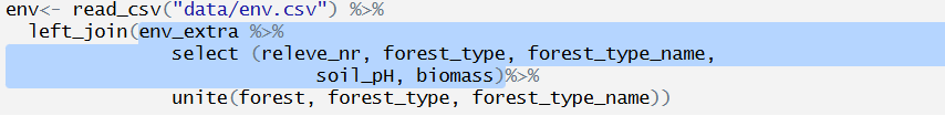
and I will prepare a merged variable called forest with code and name merged together with the unite function: 1_oak forest…
Try to send to console the pieces of the code step by step, to understand, what we are merging. Alternative way would be to save this part as another object and join it to the env file in another step. However, the approach above is more in tidyverse style.
2.1.2 spe dataset
I want to work with the spe dataset, and I want to keep information about layers, as I want to focus on the herb-layer.
spe <- read_csv ("data/spe_merged_covers.csv")Rows: 2277 Columns: 4
── Column specification ────────────────────────────────────────────────────────
Delimiter: ","
chr (1): species
dbl (3): releve_nr, layer, cover_perc
ℹ Use `spec()` to retrieve the full column specification for this data.
ℹ Specify the column types or set `show_col_types = FALSE` to quiet this message.2.1.3 traits
I also want to add some information about traits. So I will check what is available in my folder.
list.files("data") [1] "CzechVeg_tutorial.zip" "data.zip"
[3] "ellenberg_type_indicators_cz.csv" "env.csv"
[5] "env_measured.csv" "readme.txt"
[7] "remarks.cdx" "remarks.dbf"
[9] "spe.csv" "spe_juice_input.csv"
[11] "spe_merged_covers.csv" "spe_merged_covers_across_layers.csv"
[13] "species.csv" "status.csv"
[15] "table_cover.csv" "table_nomenclature.csv"
[17] "traits.csv" "tvabund.cdx"
[19] "tvabund.csv" "tvabund.dbf"
[21] "TvAdmin.cdx" "TvAdmin.dbf"
[23] "tvhabita.cdx" "tvhabita.csv"
[25] "tvhabita.dbf" "tvwin.dbf" I will import some traits e.g. plant height data, Ellenberg-type indicator values and status (origin and Red List categories). All these data are available in the PLADIAS database of the Czech flora and vegetation. I used the datasets from the download section and adjusted the format for easier data handling.
traits <- read_csv("data/traits.csv")Rows: 317 Columns: 3
── Column specification ────────────────────────────────────────────────────────
Delimiter: ","
chr (1): species
dbl (2): height, seed_mass
ℹ Use `spec()` to retrieve the full column specification for this data.
ℹ Specify the column types or set `show_col_types = FALSE` to quiet this message.indicator_values <- read_csv("data/ellenberg_type_indicators_cz.csv")Rows: 3076 Columns: 7
── Column specification ────────────────────────────────────────────────────────
Delimiter: ","
chr (1): species
dbl (6): eiv_light, eiv_temperature, eiv_moisture, eiv_reaction, eiv_nutrien...
ℹ Use `spec()` to retrieve the full column specification for this data.
ℹ Specify the column types or set `show_col_types = FALSE` to quiet this message.status <- read_csv("data/status.csv")Rows: 6098 Columns: 3
── Column specification ────────────────────────────────────────────────────────
Delimiter: ","
chr (3): species, origin, redlist
ℹ Use `spec()` to retrieve the full column specification for this data.
ℹ Specify the column types or set `show_col_types = FALSE` to quiet this message.2.2 Basic data handling
Select the columns/variables based on their names or position. Select can also be used in combination with the stringr package to identify the pattern in the names: try several options: starts_with, ends_with or a more general one contains. With the use of select in your script you can order the variables always in the same way e.g. ID, forest type, species number, productivity, even during import. And you can also rename the variables using select, to get exactly what you need.
env_extra %>%
  select(ID=releve_nr, forest_type=forest_type_name, species_nr=herbs, productivity=biomass)
# A tibble: 65 × 4
ID forest_type species_nr productivity
<dbl> <chr> <dbl> <dbl>
1 1 oak hornbeam forest 26 12.8
2 2 oak forest 13 9.9
3 3 oak forest 14 15.2
4 4 oak forest 15 16
5 5 oak forest 13 20.7
6 6 oak forest 16 46.4
7 7 oak forest 17 49.2
8 8 oak hornbeam forest 21 48.7
9 9 oak hornbeam forest 15 13.8
10 10 oak forest 14 79.1
# ℹ 55 more rowsDistinct is a function that takes your data and removes all the duplicate rows, keeping only the unique ones. There are many cases where you will really appreciate this elegant and easy way. For example, I want a list of unique PlotIDs= releve_nr, unique combinations of two categories etc. Here I want to prepare a list of forest type codes and names, and as a first step, I sorted the dataset by forest type with arrange. Note that arrange can be used also in descending order e.g. arrange (desc(forest_type)).
env_extra %>%
  arrange(forest_type) %>%
  distinct(forest_type,forest_type_name)
# A tibble: 4 × 2
forest_type forest_type_name
<dbl> <chr>
1 1 oak forest
2 2 oak hornbeam forest
3 3 ravine forest
4 4 alluvial forest When we have a large dataset, we sometimes need to create a subset of the rows/cases by filter. First we have to define upon which variable we are going to filter the rows (e.g. Forest type, soil pH…) and which values are acceptable and which are not. Here I keep only plots from a type that exactly match.
env_extra %>%
  filter(forest_type_name =="alluvial forest")
# A tibble: 11 × 22
releve_nr forest_type forest_type_name herbs juveniles coverE1 biomass
<dbl> <dbl> <chr> <dbl> <dbl> <dbl> <dbl>
1 101 4 alluvial forest 28 6 90 91.1
2 103 4 alluvial forest 35 5 80 114.
3 104 4 alluvial forest 25 11 85 188.
4 110 4 alluvial forest 37 4 95 126.
5 111 4 alluvial forest 26 10 85 84.8
6 113 4 alluvial forest 37 10 70 74.5
7 125 4 alluvial forest 25 8 95 123.
8 127 4 alluvial forest 53 6 0 176
9 129 4 alluvial forest 31 7 85 100.
10 131 4 alluvial forest 59 3 95 163.
11 132 4 alluvial forest 60 7 90 287.
# ℹ 15 more variables: soil_depth <dbl>, soil_pH <dbl>, slope <dbl>,
# altitude <dbl>, coverE3 <dbl>, radiation <dbl>, heat <dbl>,
# trans_dir <dbl>, trans_dif <dbl>, trans_tot <dbl>, eiv_light <dbl>,
# eiv_moisture <dbl>, eiv_soilreaction <dbl>, eiv_nutrients <dbl>, TWI <dbl>or those that are listed in the brackets
env_extra %>%
  filter(forest_type_name %in% c("alluvial forest", "ravine forest"))
# A tibble: 21 × 22
releve_nr forest_type forest_type_name herbs juveniles coverE1 biomass
<dbl> <dbl> <chr> <dbl> <dbl> <dbl> <dbl>
1 101 4 alluvial forest 28 6 90 91.1
2 103 4 alluvial forest 35 5 80 114.
3 104 4 alluvial forest 25 11 85 188.
4 105 3 ravine forest 12 10 80 65.5
5 106 3 ravine forest 16 0 75 33.6
6 108 3 ravine forest 28 7 70 82.3
7 110 4 alluvial forest 37 4 95 126.
8 111 4 alluvial forest 26 10 85 84.8
9 113 4 alluvial forest 37 10 70 74.5
10 114 3 ravine forest 12 6 50 71.5
# ℹ 11 more rows
# ℹ 15 more variables: soil_depth <dbl>, soil_pH <dbl>, slope <dbl>,
# altitude <dbl>, coverE3 <dbl>, radiation <dbl>, heat <dbl>,
# trans_dir <dbl>, trans_dif <dbl>, trans_tot <dbl>, eiv_light <dbl>,
# eiv_moisture <dbl>, eiv_soilreaction <dbl>, eiv_nutrients <dbl>, TWI <dbl>Or I want to filter based on some values. If I have NAs in the variable at the same time, I should specify if I want to keep these rows or not. In the example below I will keep all rows/plots where biomass is higher than 80g/m2 but I will also keep all the NAs, i.e. plots where it was not measured.
env_extra %>%
  filter(biomass>80 |is.na(biomass))
# A tibble: 17 × 22
releve_nr forest_type forest_type_name herbs juveniles coverE1 biomass
<dbl> <dbl> <chr> <dbl> <dbl> <dbl> <dbl>
1 101 4 alluvial forest 28 6 90 91.1
2 103 4 alluvial forest 35 5 80 114.
3 104 4 alluvial forest 25 11 85 188.
4 108 3 ravine forest 28 7 70 82.3
5 110 4 alluvial forest 37 4 95 126.
6 111 4 alluvial forest 26 10 85 84.8
7 120 2 oak hornbeam forest 36 6 75 98.5
8 121 2 oak hornbeam forest 30 12 80 84.7
9 122 3 ravine forest 29 6 60 102.
10 124 2 oak hornbeam forest 34 15 75 102.
11 125 4 alluvial forest 25 8 95 123.
12 127 4 alluvial forest 53 6 0 176
13 128 3 ravine forest 20 4 70 121.
14 129 4 alluvial forest 31 7 85 100.
15 130 3 ravine forest 18 5 85 238
16 131 4 alluvial forest 59 3 95 163.
17 132 4 alluvial forest 60 7 90 287.
# ℹ 15 more variables: soil_depth <dbl>, soil_pH <dbl>, slope <dbl>,
# altitude <dbl>, coverE3 <dbl>, radiation <dbl>, heat <dbl>,
# trans_dir <dbl>, trans_dif <dbl>, trans_tot <dbl>, eiv_light <dbl>,
# eiv_moisture <dbl>, eiv_soilreaction <dbl>, eiv_nutrients <dbl>, TWI <dbl>You can also filter plots in a specified range of some value.
env_extra %>%
  filter((biomass >= 40 & biomass <= 80) | is.na(biomass))
# A tibble: 20 × 22
releve_nr forest_type forest_type_name herbs juveniles coverE1 biomass
<dbl> <dbl> <chr> <dbl> <dbl> <dbl> <dbl>
1 6 1 oak forest 16 3 60 46.4
2 7 1 oak forest 17 5 70 49.2
3 8 2 oak hornbeam forest 21 1 70 48.7
4 10 1 oak forest 14 4 75 79.1
5 18 2 oak hornbeam forest 13 3 85 72.2
6 86 2 oak hornbeam forest 32 5 40 46.9
7 87 2 oak hornbeam forest 34 9 65 42.9
8 99 2 oak hornbeam forest 18 6 85 64.8
9 102 2 oak hornbeam forest 37 13 65 57.4
10 105 3 ravine forest 12 10 80 65.5
11 109 2 oak hornbeam forest 25 9 50 60.7
12 112 2 oak hornbeam forest 32 14 60 58.4
13 113 4 alluvial forest 37 10 70 74.5
14 114 3 ravine forest 12 6 50 71.5
15 115 3 ravine forest 23 2 70 54.6
16 116 3 ravine forest 16 3 45 64.5
17 117 2 oak hornbeam forest 31 7 55 54.7
18 118 2 oak hornbeam forest 8 5 45 66.2
19 123 3 ravine forest 34 11 70 53.6
20 126 2 oak hornbeam forest 27 7 65 72.9
# ℹ 15 more variables: soil_depth <dbl>, soil_pH <dbl>, slope <dbl>,
# altitude <dbl>, coverE3 <dbl>, radiation <dbl>, heat <dbl>,
# trans_dir <dbl>, trans_dif <dbl>, trans_tot <dbl>, eiv_light <dbl>,
# eiv_moisture <dbl>, eiv_soilreaction <dbl>, eiv_nutrients <dbl>, TWI <dbl>Similarly, you can for example, filter plots based on their plot size. The example below is not working on our dataset, but it comes in useful in large EVA exports. Here I keep grassland plots in the range 10-100 m2, forest plots between 100-1000 m2 and I keep the plots without a specified plot size.
env %>%
  filter(
    (habitat == "grassland" & plot_size >= 10 & plot_size <= 100) |
    (habitat == "forest" & plot_size >= 100 & plot_size <= 1000) |
    is.na(plot_size)
  )
Mutate Often, you need to prepare new variables, based on the existing variables, filled with some value (number or string) or you need to rewrite the values of a variable. For this, you can use the mutate function.
Here I prepare new variable by summing two columns:
env_extra %>%
  mutate(herblayer_richness = herbs+juveniles) %>%
  select(releve_nr, herblayer_richness, herbs, juveniles)
# A tibble: 65 × 4
releve_nr herblayer_richness herbs juveniles
<dbl> <dbl> <dbl> <dbl>
1 1 38 26 12
2 2 16 13 3
3 3 15 14 1
4 4 20 15 5
5 5 14 13 1
6 6 19 16 3
7 7 22 17 5
8 8 22 21 1
9 9 19 15 4
10 10 18 14 4
# ℹ 55 more rowsOr I can define new variable based on some conditions with ifelse (first I state what happens if the condition is met (here “low”), then what happens with the rest (“high”) and I can nest more ifelse statements)
env_extra %>%
  mutate(productivity = ifelse(biomass<60,"low","high")) %>%
  select (releve_nr, forest_type_name, productivity, biomass) %>%
  print(n=20)
# A tibble: 65 × 4
releve_nr forest_type_name productivity biomass
<dbl> <chr> <chr> <dbl>
1 1 oak hornbeam forest low 12.8
2 2 oak forest low 9.9
3 3 oak forest low 15.2
4 4 oak forest low 16
5 5 oak forest low 20.7
6 6 oak forest low 46.4
7 7 oak forest low 49.2
8 8 oak hornbeam forest low 48.7
9 9 oak hornbeam forest low 13.8
10 10 oak forest high 79.1
11 11 oak forest low 7.4
12 14 oak hornbeam forest low 14.2
13 16 oak hornbeam forest low 26.2
14 18 oak hornbeam forest high 72.2
15 28 oak forest low 29.7
16 29 oak hornbeam forest low 37.9
17 31 oak forest low 14.9
18 32 oak hornbeam forest low 19.2
19 36 oak hornbeam forest low 3.3
20 41 oak hornbeam forest low 26.9
# ℹ 45 more rowsor with case_when I can define a set of conditions and assign the value to each of them
env_extra %>%
  mutate(productivity = case_when(biomass <= 60 ~ "low",
                                  biomass > 60 ~ "high"))
Join functions are used either to append new information (left_join, inner_join, full_join) or to filter our dataset (semi_join, anti_join) based on the comparison with another dataset. We always need to have some common variables which have exactly the same name or we have to specify using by which variables are equivalent in the two datasets e.g. left_join(traits, by = c("species"= "taxon"). In most cases we will use left_join which is used for appending information from another file, without changing the number of rows in the original file. If the information is not available, the value will be NA.

For more on join functions see here.
2.3 Summarise
Using the group_by() function, we can define how the data should be arranged into groups. Then we can proceed with asking questions about these groups. The basic function of summarising information is to count the number of rows, and we do not have to even specify the grouping variable separately, only within count. Count returns numbers stored as n, but we can also directly rename it e.g. count (forest_type_name, name= “frequency”).
env_extra %>%
  count(forest_type_name)
# A tibble: 4 × 2
forest_type_name n
<chr> <int>
1 alluvial forest 11
2 oak forest 16
3 oak hornbeam forest 28
4 ravine forest 10But we can explore the data much more. For example calculate mean values per vegetation type.
env %>%
  group_by(forest) %>%
  summarise(mean_biomass = mean(biomass))
# A tibble: 4 × 2
forest mean_biomass
<chr> <dbl>
1 1_oak forest 26.7
2 2_oak hornbeam forest 44.4
3 3_ravine forest 88.7
4 4_alluvial forest 139. We might produce a table with summary statistics like min, mean, max for several variables per forest type at once, listing both the variables and functions which should be applied.
env_extra %>%
  arrange(forest_type,forest_type_name) %>%
  group_by(forest_type,forest_type_name) %>%
  summarise(across(c(coverE1, biomass, coverE3, soil_pH),
      list(
        min  = ~min(.x, na.rm = TRUE),
        mean = ~mean(.x, na.rm = TRUE),
        max  = ~max(.x, na.rm = TRUE))))
`summarise()` has grouped output by 'forest_type'. You can override using the
`.groups` argument.# A tibble: 4 × 14
# Groups: forest_type [4]
forest_type forest_type_name coverE1_min coverE1_mean coverE1_max biomass_min
<dbl> <chr> <dbl> <dbl> <dbl> <dbl>
1 1 oak forest 8 37.1 75 7.4
2 2 oak hornbeam for… 7 52.6 85 3.3
3 3 ravine forest 45 67.5 85 33.6
4 4 alluvial forest 0 79.1 95 74.5
# ℹ 8 more variables: biomass_mean <dbl>, biomass_max <dbl>, coverE3_min <dbl>,
# coverE3_mean <dbl>, coverE3_max <dbl>, soil_pH_min <dbl>,
# soil_pH_mean <dbl>, soil_pH_max <dbl>Rather than tables, we can produce graphical outputs, such as boxplots. See our study materials for basicand advanced ggplot2 functions.
env %>%
  arrange(forest) %>%
  select(forest, cover_herbs=cov_herbs, biomass, cover_trees =cov_trees, soil_pH) %>%
  tidyr::pivot_longer(
    cols = c(cover_herbs, biomass, cover_trees, soil_pH),
    names_to = "variable",
    values_to = "value")%>%
  ggplot(aes(x = forest, y = value, fill=forest)) +
  geom_boxplot() +
  facet_wrap(~ variable, scales = "free_y") +
  theme_bw() +
  theme(legend.position = 'none')+
  theme(axis.text.x = element_text(angle = 45, hjust = 1))+
  labs(x = NULL) +
  labs (y = NULL)
We might be interested in species richness relationship with several factors. Below is an example of herb-layer species richness and biomass. At first I need to calculate the species richness in the spe file. And as an output I want to plot this with different colours for different forest types but keep the regression line for the whole dataset.
spe %>%
  filter(layer %in% c(6, 7)) %>%
  count(releve_nr, name = "herblayer_richness") %>%
  left_join(env %>%
              select(releve_nr, biomass, forest), by = "releve_nr") %>%
  ggplot(aes(x = sqrt(biomass), y = herblayer_richness)) +
  geom_point(aes(colour = forest), size = 2, alpha = 0.8) +
  geom_smooth(method = "lm", se = TRUE, colour = "black") +
  theme_bw() +
  labs(
    x = "sqrt Biomass",
    y = "Herb-layer species richness",
    colour = "Forest type"
  )
`geom_smooth()` using formula = 'y ~ x'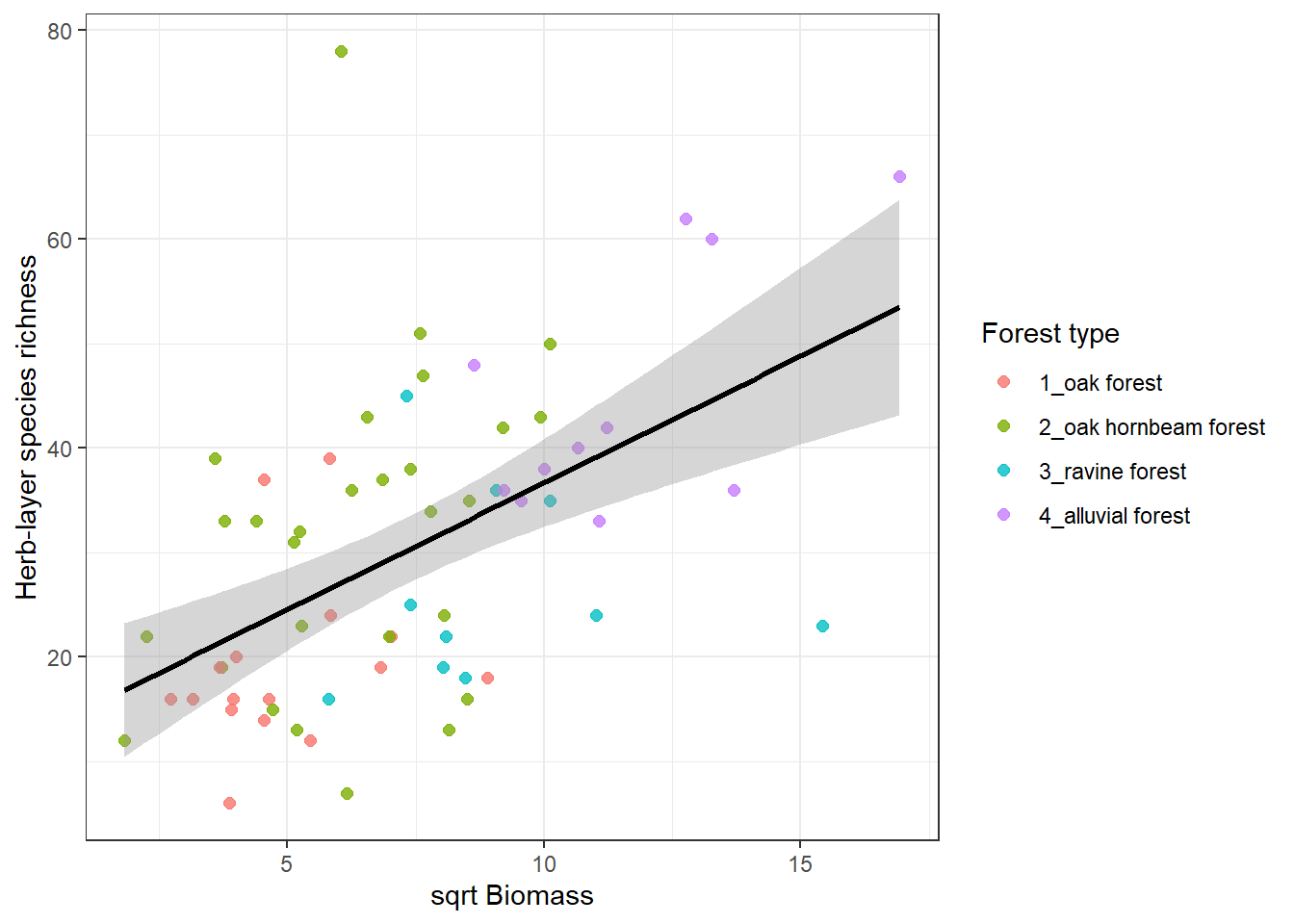
Proportions of endangered or alien species in forest type. I will first look at the numbers of these species, here on example of redlist i.e. endangered species. I just one to see average number of redlist species per forest type.
spe%>%
  left_join(spe %>%
              left_join(status)%>%
              filter(!is.na(redlist))%>%
              count(releve_nr, name="richness_redlist"))%>%
  left_join(spe %>%
              summarise(richness_all = n_distinct(species),
                        .by = releve_nr))%>%
  distinct(releve_nr,richness_redlist,richness_all)%>%
  mutate(richness_redlist = replace_na(richness_redlist, 0))%>%
  mutate(richness_redlist_perc= richness_redlist/richness_all*100)%>%
  left_join(env%>% select(releve_nr, forest))%>%
  summarise(redlist_mean_perc = mean(richness_redlist_perc), .by=forest)%>%
  arrange(forest)
Joining with `by = join_by(species)`
Joining with `by = join_by(releve_nr)`
Joining with `by = join_by(releve_nr)`
Joining with `by = join_by(releve_nr)`# A tibble: 4 × 2
forest redlist_mean_perc
<chr> <dbl>
1 1_oak forest 7.95
2 2_oak hornbeam forest 6.45
3 3_ravine forest 5.39
4 4_alluvial forest 2.12But I can also ask about diferences in abundances of some plant groups. What is the proportion of cover of alien species relative to total cover in different forests? I will again use the function we used for cover combination during import from Turboveg.
combine_cover <- function(x){
  while (length(x)>1){
    x[2] <- x[1]+(100-x[1])*x[2]/100
    x <- x[-1]
  }
  return(x)
}spe%>%
left_join(spe %>%
left_join(status)%>%
filter(origin %in% c("arch","neo"))%>%
summarize(cover_alien = combine_cover(cover_perc),
.by=releve_nr))%>%
left_join(spe %>%
summarize(cover_total = combine_cover(cover_perc),
.by=releve_nr))%>%
distinct(releve_nr, cover_alien, cover_total)%>%
mutate(cover_alien = replace_na(cover_alien, 0))%>%
mutate(cover_alien_perc= cover_alien/cover_total*100)%>%
left_join(env%>% select(releve_nr, forest))%>%
summarise(alien_cover_mean_perc = mean(cover_alien_perc), .by=forest)%>%
arrange(forest)Joining with `by = join_by(species)`
Joining with `by = join_by(releve_nr)`
Joining with `by = join_by(releve_nr)`
Joining with `by = join_by(releve_nr)`# A tibble: 4 × 2
forest alien_cover_mean_perc
<chr> <dbl>
1 1_oak forest 0.0188
2 2_oak hornbeam forest 1.24
3 3_ravine forest 3.11
4 4_alluvial forest 3.44 2.4 Community weighted means
Summarise is often used for getting so-called community means or community weighted means. For example we have traits for individual species and we want to calculate a mean for each site and compare it. We can also consider to use abundance to weight the result. This is called community weighted mean and it simply gives higher importance to those species that are more abundant and lower importance to the rare once. Here the abundance is approximated as percentage cover in the site. The example below compares mean plant height both weighted and unweighted. To have meaningful values, I looked just at the herb-layers species.
spe %>%
  left_join(traits) %>%
  filter(layer==6)%>%
  summarise(meanHeight= mean(height, na.rm=T),
            meanHeight_weighted = weighted.mean(height, cover_perc, na.rm = TRUE),
            .by=releve_nr)
Joining with `by = join_by(species)`# A tibble: 65 × 3
releve_nr meanHeight meanHeight_weighted
<dbl> <dbl> <dbl>
1 1 0.348 0.322
2 2 0.454 0.494
3 3 0.430 0.391
4 4 0.570 0.522
5 5 0.563 0.514
6 6 0.562 0.573
7 7 0.491 0.553
8 8 0.458 0.699
9 9 0.476 0.493
10 10 0.539 0.560
# ℹ 55 more rows2.5 Ellenberg indicator values
In the same way we can calculate community means across more variables. Here we will try the Ellenberg indicator values (abbreviated as EIV, measures of species demands for the particular factors, the higher value mean higher demands or affinity to habitats with higher values of these environmental factors). We will apply them just for presences of species, so no weights. Therefore we do not need to care that much for the differences among layers. However, we will keep each species only once (list of unique species for each plot), so we will remove information about layers first and use distinct. Alternative is to add #filter(Layer==6)%>% if we want to focus on herb-layer only
spe %>%
  left_join(indicator_values) %>%
  select(-c(layer,cover_perc))%>%
  distinct()%>%
  group_by(releve_nr)%>%
  summarise(across(starts_with("eiv"), ~ mean(.x, na.rm = TRUE)))
Joining with `by = join_by(species)`# A tibble: 65 × 7
releve_nr eiv_light eiv_temperature eiv_moisture eiv_reaction eiv_nutrients
<dbl> <dbl> <dbl> <dbl> <dbl> <dbl>
1 1 5.08 5.56 4.64 6.54 4.95
2 2 4.87 5.2 4.8 5 4.33
3 3 4.87 5.13 4.8 5 4.4
4 4 5.32 5.53 4.47 5.79 4.26
5 5 6.07 5.57 4.14 5.57 3.86
6 6 5.72 5.56 4.5 6.44 5.22
7 7 5.75 5.45 4.45 6.25 4.95
8 8 5.13 5.39 4.70 5.48 4.70
9 9 5.38 5.67 4.48 5.95 4.43
10 10 6.38 5.88 3.69 6.19 3.88
# ℹ 55 more rows
# ℹ 1 more variable: eiv_salinity <dbl>Boxplots of Ellenberg-type indicator values can be produced for example like this: You can try again sending parts of the script to console, always adding new part and see what happens.
spe %>%
  left_join(indicator_values) %>%
  select(-c(layer, cover_perc)) %>%
  distinct() %>%
  group_by(releve_nr) %>%
  summarise(across(starts_with("EIV"), ~ mean(.x, na.rm = TRUE))) %>%
  left_join(env %>% select(releve_nr, forest))%>%
  pivot_longer(
    cols = starts_with("EIV"),
    names_to = "EIV_variable",
    values_to = "value")%>%
  ggplot(aes(x = forest, y = value, fill = forest)) +
  geom_boxplot() +
  facet_wrap(~ EIV_variable, scales = "free_y") +
  theme_bw()+
  theme(legend.position = 'none')+
  theme(axis.text.x = element_text(angle = 45, hjust = 1))+
  labs(x = NULL) +
  labs (y = NULL)
Joining with `by = join_by(species)`
Joining with `by = join_by(releve_nr)`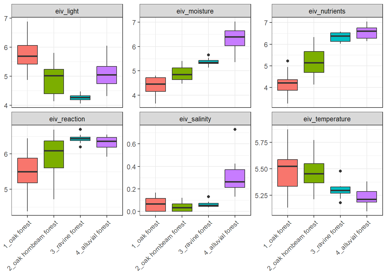
2.6 Visualisation
Visualisation is not part of the tutorial at the moment, but we recommend our study materials for basic and advanced ggplot2 functions. However, we plan to include more examples in the future releases.